Observability

Observability is how understandable the internal state of a sytem from the outputs it emits. Normally, a software system has limited inputs and outputs. For example, a service has API requests as its inputs and responses as its outputs. These responses are not enough to understand the internal state of any complex system. For example, if it takes a long time for a service to respond to a request, it could be because the service has too much traffic, a bug was introduced from a recent code change, or critical hardware failed. From a single response, there is no way of to know if the issue has occurred in the past or this is the first time it has happened.

We must instrument our software to emit additional outputs or signals that grant more information about the internal state. Instrumentation is the practice of inserting signal producing code into applications. These signals increase the observability of our software. There are 4 types of signals that engineers can instrument their software to emit: logs, metrics, traces, and profiles.

Logs

Logs are human readable messages emitted by a system. Each new log message is appended to existing logs. Log levels are used to categorize log messages by importance. Log levels vary by logging library, but the popular Log4j library has 6 log levels, listed below in order of increasing importance.

Table TODO. Log4j log levels in increasing severity.

Log Level	Description
Trace	Used for fine grain debugging.
Debug	Used for debugging.
Info	Used for informational messages.
Warning	Used for messages that are not errors, but may indicate an issue.
Error	Used for errors that may allow the application to continue running.
Fatal	Used for errors that will cause the application to abort.

Most logging libraries have similar log levels. Log messages with a log level below the configured logger log level will not be written. This is useful since more messages are helpful for debugging but is overwhelming for production.

import logging

def get_logger(name):
    logger = logging.getLogger(name)
    handler = logging.StreamHandler()
    formatter = logging.Formatter('%(name)s %(asctime)s %(levelname)s %(message)s')
    handler.setFormatter(formatter)
    logger.addHandler(handler)

    return logger

logger = get_logger('my_logger')
logger.setLevel(logging.INFO)
logger.debug('This message will NOT be written.')
logger.info('This message will be written.')

my_logger 2024-02-21 07:19:17,169 INFO This message will be written.

There are 2 types of messages that logging software can emit.

Unstructured logs

The message is a line of text. Usually, the line of text is a sentence that describes an event that has occurred. Best practice is to include the logger name, timestamp, log level, and other metadata in the log message.

2023-11-26T03:02:15,015Z INFO Hello, world! Requested by user 123.

Structured logs

Each record is an object and has a format like JSON or XML. Rather than put the timestamp, log level, and other metadata in the log message, they are put in separate fields. The message itself can be split across multiple fields.

{
  "level": "INFO",
  "message": "Hello World!",
  "timestamp": "2023-11-26T03:02:15.015Z",
  "user_id": 123
}

The advantage of structured logs is that they are easier to search. For example, suppose we want to find the stack traces for all NullPointerExceptions that occurred in the past 7 days. For unstructured logs, each logged NullPointerException starts with an ERROR message containing NullPointerException. The stack trace is spread across multiple lines. We need a shell command or script that executes the following 3 steps.

1. Filter all log messages that occur in the past 7 days.

2. Find all log messages that contain the string “NullPointerException”.

3. Extract the stack trace from subsequent log messages.

For structured logs, each logged NullPointerException is a JSON object with a stack_trace field. Many cloud providers have log query languages such as CloudWatch Logs Insights and Google Cloud Log Explorer that support these type of queries. Finding the desired stack traces is a single log query that has 3 parts.

1. Filter by timestamp to the past 7 days.

2. Filter by message to include “NullPointerException”.

3. Retrieve the stack_trace field.

What to Log

Before deciding what to log, it helps to understand when logs are looked at. Log are examined almost exclusively to debug issues. Therefore, log errors, failures, and any risky event. Log the cause of the error or failure, if available. Logs should be as detailed as possible. After an incident occurs, you cannot go back in time to add more logs.

Log important events, which are not errors, that occur in a system. In general, the log level should be Info and above. Info log messages help form a historical record of important events that have occurred in the system. These log messages provide context for future debugging.

These guidelines serve as a minimal starting point. Depending on the use case, you may want to log more. Avoid the temptation to log everything. This will make logs unreadable and is expensive.

Never log sensitive data.

• Personally identifiable information (PII) such as names, addresses, and government identification numbers.

• Payments information such as credit card number and bank account numbers.

• Security information such as passwords, encryption keys, access tokens, and other secrets.

Leaks of sensitive data will result in lost trust with customers and potentially financial penalties or legal action. Due to the damage that leaks of sensitive data can cause, it has a higher standard for transmission and storage. If logs contains sensitive data, now the entire logging system must meet this higher standard. Logs need to be encrypted and access restricted which adds friction. This is antithetical to the goal of aiding debugging. Better to not log sensitive data at all.

Important

Keep logging software up to date. The Log4Shell vulnerability in December 2021 has made it clear that logging libraries potential surfaces for attackers to exploit.

Instrumentation

How logging is instrumented depends on the programming language and the logging library. Some logging libraries allow the logger to be constructed with a single line of code. For example, the @Log4 annotation in Lombok will create a logger in the variable log for the class. In Python, the standard docs recommend to create a logger at the top of each module using the below line.

logger = logging.getLogger(__name__)
logger

<Logger __main__ (WARNING)>

The logger name should reflect the class or module hierarchy and include the class or module name. The name change makes it easier to identify the source of the log message. If possible, separate logs into different streams. For example, as a service processes each request, the logs associated with that request should be written to a separate stream. This makes it easier to follow the logs for a single rquest than the alternative where logs from all requests are interleaved.

Logs should be continuously streamed over network to a centralized log aggregator, popularly in the cloud. This includes not just application logs but operating system logs, server logs, load balancer logs, and other logs from the infrastructure around the application. The log aggregator persists logs outside of the machine that generates them. This is important to avoid losing logs if the machine crashes. The log aggregator is a single place to search and analyze logs. Log aggregators often index the logs to speed up searches compared to simply greping log files.[1]

Do not retain logs infinitely. Because logs have primarily string content, they are expensive to store and search. Common retention periods are on the order of months. If you need information about a system from further back, consider using the next signal type.

Metrics

Metrics are numerical measurements of a system. Each metric data point (or datum) is a tuple consisting of the metric name, the numerical value, the units, a timestamp, and a set of key-value pairs called dimensions or labels[2]. Depending on the observability system, data points may have extra fields.

from dataclasses import dataclass
from datetime import datetime
from typing import Dict

@dataclass
class DataPoint:
    metric_name: str
    metric_value: float  # or int if the metric is a count
    unit: str
    timestamp: datetime
    dimensions: Dict[str, str]

Together, these datapoints form a time series \(x = (x_1, x_2, \dots, x_n)\). The time series is not necessarily equally spaced. For example, a duration metric that measures the time to respond for a service will have a time series with a datapoint for each request. Depending on the traffic, the time between datapoints will vary.

Retaining the individual datapoints is expensive and impractical to use. These raw time series can be aggregated using statistics. The statistic divides time into intervals of length \(T\) and computes a single values based on the datapoints that occur in each interval. The final result is a time series with equally spaced datapoints.

Average (or Mean)

For each time interval interval, average the values of all datapoints. For measurement style metrics, this statistic usually makes the most sense. For example, if the metric is the disk usage of a database, using an average statistic over a 5 minute period shows the average disk usage across the 5 minutes.

Max

For each time interval, take the maximum value of all datapoints.

Min

For each time interval, take the minimum value of all datapoints.

Percentile

For each time interval, take the \(a\)th percentile of all datapoints. Often this is abbreviated as p\(a\). For example, p99 is the 99th percentile.

• p0 is the minimum.

• p50 is the median.

• p100 is the maximum.

Percentile is useful for capturing the tails of a distribution. For example, a useful statistic for services is the p99 of latency. This statistic shows the worst latency 1% of clients experience.

Sample Count

For each time interval, count the number of datapoints. This statistic is useful to count the number of events that have occurred from a measurement type metric. For example, if the metric is the response latency, the sample count statistic over a 5 minute period is the number of requests that were made every 5 minutes.

Sum

For each time interval, sum the values of all datapoints. For count style metrics, this statistic usually makes the most sense. For example, if the metric is the number of errors, using a sum statistic over a 5 minute period shows the total number of errors every 5 minutes.

There are many more possible statistics. For example, AWS CloudWatch has 12 statistics. Below is an example of a time series with 100 datapoints and the average, max, median, and min statistics.

%config InlineBackend.figure_format = 'retina'
import matplotlib.pyplot as plt
import numpy as np

np.random.seed(0)
x = 100 * np.random.uniform(0, 1, 100)
periods = np.arange(0, 100, 5)

plt.plot(x, label='Data', alpha=0.5)
plt.plot(periods, np.mean(x.reshape(-1, 5), axis=1), label='Average')
plt.plot(periods, np.max(x.reshape(-1, 5), axis=1), label='Max')
plt.plot(periods, np.median(x.reshape(-1, 5), axis=1), label='Median')
plt.plot(periods, np.min(x.reshape(-1, 5), axis=1), label='Min')
plt.xlabel('Time (min)')
plt.ylabel('CPU Utilization (%)')
plt.legend(loc='upper right')

<matplotlib.legend.Legend at 0x7f77b00d3290>

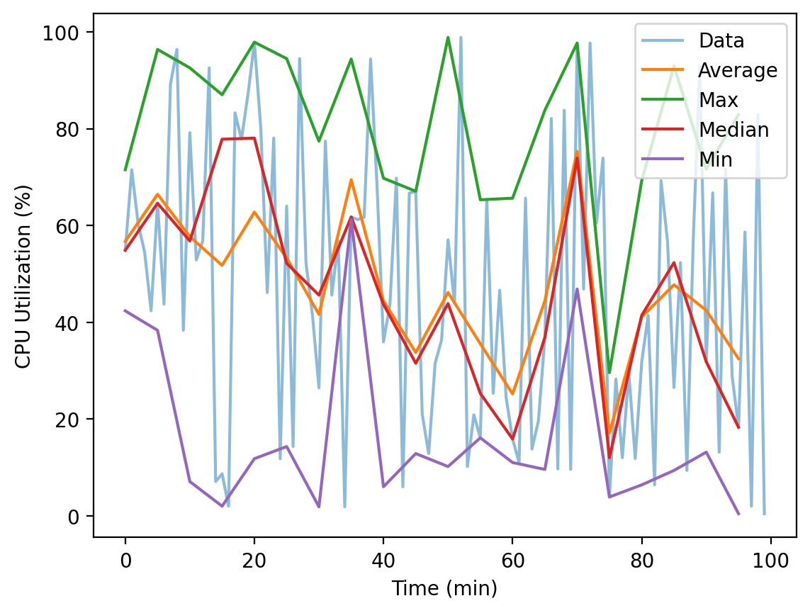
Each statistic loses information from the original time series. Sometimes it can be helpful to look at the distribution of datapoints summarized as a histogram.

What to Measure

The following metrics should be measured for all services.

• Dependencies. If a service \(A\) depends on another service \(B\), measure the inputs and outputs \(B\) receives from and sends to \(A\). Dependencies can also be databases, queues, and caches. Some common metrics are given below.

  • Number of requests

  • Number of errors

  • Latency

  It can be helpful to add these metrics

• Resources. Aim to measure the utilization of all compute, memory, storage, and other resources as percentages of the total capacity. It is important to use percentages since the total capacity may be elastic. Depending on the programming language, there may be additional resources that need to be measured, such as heap space for Java or goroutines for Go. Some common metrics are given below.

  • CPU utilization

  • Memory utilization

  • Disk utilization

  • Network utilization

• Served Traffic. Just as a servier’s inputs and outputs it sends to and receives to its dependencies ought to be measured, measure the inputs and outputs your service receives from and sends to its clients. This is especially important for services that are exposed to the public. The common metrics are the same as those for dependencies.

These guidelines serve as a minimal starting point. Depending on the use case, you may want to measure more. In particular, metrics are useful for tracking long term trends. For example, measuring the number of users that sign up each day allows the business to track how fast it is growing.

See also

Further reading: The Four Golden Signals

Instrumentation

How metrics are instrumented depends on the programming language and the metrics library. Ideally, the metrics library allows engineers to emit metrics with a single line of code. In languages with annotations or decorators, metrics libraries can provide annotations or decorators that can be applied to functions to emit metrics at the end of the function. For example, the Python client of Prometheus, an open source metrics library, has decorators to time functions and emit the duration as a metric.

from prometheus_client import Summary
s = Summary('request_latency_seconds', 'The time it takes to respond to a request in seconds.')

@s.time()
def f():
    pass

f()
s.collect()[0]

Metric(request_latency_seconds, The time it takes to respond to a request in seconds., summary, , [Sample(name='request_latency_seconds_count', labels={}, value=1.0, timestamp=None, exemplar=None), Sample(name='request_latency_seconds_sum', labels={}, value=1.152000010051779e-06, timestamp=None, exemplar=None), Sample(name='request_latency_seconds_created', labels={}, value=1708499957.9172335, timestamp=None, exemplar=None)])

Like with logs, metrics should be exported to an external metrics collector. Often this is done by running a metrics agent process on the machine that transmits metrics over a network to the metrics collector. The metrics collector persists metrics in a database, outside the machine that generated the metrics, and indexes them for fast search. There are 2 ways metrics can be exported.

Pull

The metrics collector makes a request, usually HTTP, to the metrics agent to collect metrics. The metrics agent replies with the metrics. An example of a pull based system is Prometheus.

Push

The metrics agent sends metrics, usually over UDP, to the metrics collector. An example of push based system is Graphite.

Pull based systems are easier to control and debug since there is a clear distinction between the metrics collector and the metrics agent. Push based systems ensure that metrics are always sent even for short lived processes. Push based system also have an easier time broadcasting metrics to multiple collectors, although it becomes harder to manage metric collection capacity.

See also

Further reading: Push Vs. Pull In Monitoring Systems

Metrics should be retained for years. Metrics take up less space than logs and so do not need to be deleted as often. Retaining metrics for years allows you to analyze long term trends. One trick is to lose granularity over time. For example, we could keep

• up to 1 minute period metrics for the past 1 day

• up to 5 minute period metrics for the past 1 year

• up to 1 hour period metrics for older than 1 year.

After all, it is rare to analyze metrics from more than 1 year ago for minute by minute changes.

Distributed Tracing

Distributed tracing tracks requests as they move through a distributed system. The entire story of a request is captured in a trace. The story is told in spans or segments. Each span represents a single unit of work or an operation. A span has a span id, timing information, error data, the request, the response, and the parent span (more on this later). Depending on the distributed tracer, spans may have more attributes.

Since requests can lead to further requests, spans can have other spans as children. Thus, a trace is a tree of spans. To maintain the lineage of spans, contexts containing the trace id, a unique identifier for each trace, and previous span are added to requests. The previous span is the parent of any new spans.

For example, suppose we have a service consisting of an API gateway, a backend service, a write through cache, and a database. All incoming requests hit the API gateway which routes them to the backend. The backend first looks up data in its cache. If there is a cache miss, then the backend checks the database.

When a request reaches the API gateway, the distributed tracer creates a trace id and top level Span 1. The API gateway forwards the request with the context to the backend. The tracing system creates Span 2 for backend service asa child of Span 1. The backend tries to find the data in the cache but fails. Span 3 for the cache is a child of Span 2. Finally, the backend checks the database which succeeds. The entire trace is shown below.

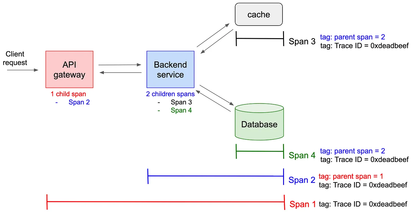
Fig. 1 An example service with the trace for a single request. Image source.

There are 2 common ways to visualize traces.

• Traces can be visualized as a graph where each span is a node and the parent-child relationship is an edge. This graph will be directed and acyclic since the trace is a tree.

• Traces can be visualized as a timeline. The x-axis is time while the spans are listed on the y-axis by order of appearance. The span is drawn as a horizontal line from the start time to the end time.cThe parent-child relationship is visible since the child span is drawn beneath the parent span. Moreover, child spans take less horizontal space than parent spans since the parent span is open the entire duration of the child span.

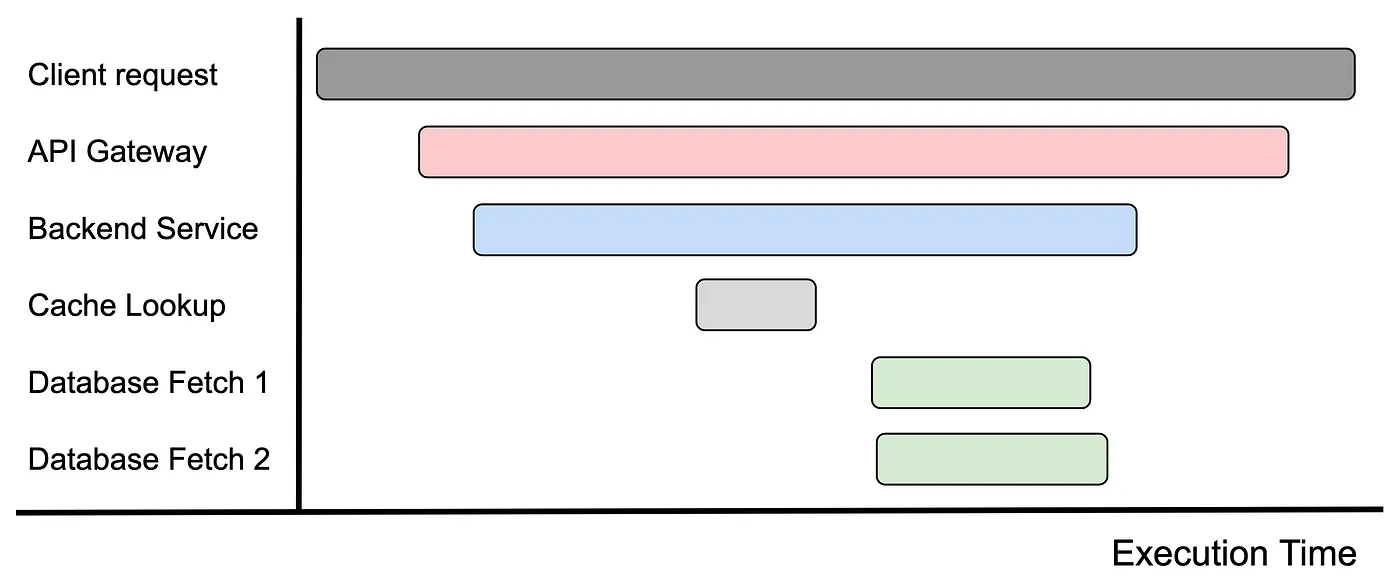
Fig. 2 Timeline for a single trace of an example service. Image source.

See also

Further reading: Distributed Tracing at Strava

What to Trace

While you can trace every request that enters a system, this is likely unnecessary. The majority of traces will be of successfully handled requests. A better approach is sampling, processing and exporting a subset of traces. Ideally, a sampler reduces costs while keeping interesting traces. These are opposing properties a sampler must balance.

Head sampling

The decision to trace is made when a request enters the system. Head sampling includes the most common type of sampling, random sampling which traces only a proportion of requests.

Head sampling is simpler to understand and implement but cannot achieve certain desirable things. For example, a common wish is to sample all traces which end in an error. Or sample all traces that take longer than \(T\) time. Head sampling decides to sample traces before error or duration information is available.

Tail sampling

The decision to trace is made after the whole trace is completed. Any sampling strategy can be expressed using tail sampling, but the implementation is harder. Spans are created across the distributed system but must somehow be examined by the tail sampler. As a consequence, many distributed tracing systems do not support tail tracing.

Samplers are not mutually exclusive. For example, a random sampler which traces 5% of requests could be paired with a tail sampler that keeps traces that end in error.

Instrumentation

How distributed tracing is instrumented depends on the programming language and the tracing library. Ideally, tracing library allows engineers to trace with a single line of code. In languages with annotations or decorators, trace libraries can provide annotations or decorators that can be applied to functions to create a span. For example, the Python API for Open Telemetry, an open source observability library, has decorators to trace functions.

from opentelemetry import trace
from opentelemetry.sdk.trace import TracerProvider
from opentelemetry.sdk.trace.export import ConsoleSpanExporter, SimpleSpanProcessor

trace.set_tracer_provider(TracerProvider())
trace.get_tracer_provider().add_span_processor(
    SimpleSpanProcessor(ConsoleSpanExporter())
)
tracer = trace.get_tracer(__name__)

@tracer.start_as_current_span('handle_request')
def handle_request():
    call_external_service()
    call_database()

@tracer.start_as_current_span('external_call')
def call_external_service():
    pass

@tracer.start_as_current_span('database_call')
def call_database():
    pass


handle_request()

{
    "name": "external_call",
    "context": {
        "trace_id": "0x9f07d5c5a8965259905683d02e184e06",
        "span_id": "0xd3c5e7d1ab4b7512",
        "trace_state": "[]"
    },
    "kind": "SpanKind.INTERNAL",
    "parent_id": "0x10851c21698563fd",
    "start_time": "2024-02-21T07:19:17.956239Z",
    "end_time": "2024-02-21T07:19:17.956250Z",
    "status": {
        "status_code": "UNSET"
    },
    "attributes": {},
    "events": [],
    "links": [],
    "resource": {
        "attributes": {
            "telemetry.sdk.language": "python",
            "telemetry.sdk.name": "opentelemetry",
            "telemetry.sdk.version": "1.22.0",
            "service.name": "unknown_service"
        },
        "schema_url": ""
    }
}

{
    "name": "database_call",
    "context": {
        "trace_id": "0x9f07d5c5a8965259905683d02e184e06",
        "span_id": "0x5cfecd1e550252cc",
        "trace_state": "[]"
    },
    "kind": "SpanKind.INTERNAL",
    "parent_id": "0x10851c21698563fd",
    "start_time": "2024-02-21T07:19:17.956836Z",
    "end_time": "2024-02-21T07:19:17.956847Z",
    "status": {
        "status_code": "UNSET"
    },
    "attributes": {},
    "events": [],
    "links": [],
    "resource": {
        "attributes": {
            "telemetry.sdk.language": "python",
            "telemetry.sdk.name": "opentelemetry",
            "telemetry.sdk.version": "1.22.0",
            "service.name": "unknown_service"
        },
        "schema_url": ""
    }
}

{
    "name": "handle_request",
    "context": {
        "trace_id": "0x9f07d5c5a8965259905683d02e184e06",
        "span_id": "0x10851c21698563fd",
        "trace_state": "[]"
    },
    "kind": "SpanKind.INTERNAL",
    "parent_id": null,
    "start_time": "2024-02-21T07:19:17.956193Z",
    "end_time": "2024-02-21T07:19:17.957342Z",
    "status": {
        "status_code": "UNSET"
    },
    "attributes": {},
    "events": [],
    "links": [],
    "resource": {
        "attributes": {
            "telemetry.sdk.language": "python",
            "telemetry.sdk.name": "opentelemetry",
            "telemetry.sdk.version": "1.22.0",
            "service.name": "unknown_service"
        },
        "schema_url": ""
    }
}

Like logs and metrics, traces should be exported to a centralized trace collector. The trace collector persists traces outside of the machine that generated them and indexes them for fast search. The trace collector should also be able to visualize traces as graphs and timelines. The trace collector should also be able to search for traces based on the trace id, the span id, and the attributes of the spans.

Traces can be retained for longer than logs. A trace occurs only when entering different service components while log messages are emitted more frequently. Thus, traces take up less space than logs and so do not need to be deleted as often. With sampling, the number of traces can be reduced further. Errored traces should always be sampled for later debugging, but successful traces can be sampled at a lower rate.

Continuous Profiling

Profiling a type of program analysis that measures the performance of a program.

CPU profiling is the most common type of profiling.

Flame graphs are a popular way of visualizing profiles.

https://www.infoq.com/presentations/profiles-continuous-profiling-observability/

What to Profile

Services

Instrumentation

When to Use Each Signal

---

[1]

Log queries are also easier to write than piped grep commands.

[2]

Observe that the data structure of a metric data point is similar to a structured log. Some observability systems take advantage of this by emitting metrics via logs.